Closing Time vs Expected (CTvE)
Quantifying defender post-throw execution by measuring how quickly players close on the ball relative to expectation.
Introduction
1.1 Motivation
In NFL pass defense, a defender’s pre-throw diagnosis and post-throw execution determines whether a play results in a completion, a pass breakup, or a turnover. Currently, defensive backs are judged on statistics like targets, yards/touchdowns allowed, passes defensed, and separation. These metrics capture outcomes, rather than execution. These metrics are often skewed by quarterback decision-making, quarterback execution, and receiver skill. They don’t show core defender traits that define coverage quality such as recognition, technique, and speed. Player tracking data allows us to move past outcome-based evaluation and quantify the process of pass defense.
1.2 Goal of the Project
The goal of this project is to build a metric, Closing Time vs Expected (CTvE), that quantifies how effectively defenders break on the football once it is thrown. CTvE separates a defender’s expected arrival time, predicted by a machine learning model using contextual and physical features, from their actual arrival time measured directly from player-tracking data. The metric captures how much faster or slower a defender closes relative to expectation, allowing for a better evaluation of post-throw execution by the defender.
Player-tracking data also allows CTvE to be decomposed into four underlying factors: anticipation, reaction ability, closing speed, and pursuit efficiency. Together, these components help explain why a player over- or underperforms their expected closing time. This analysis filters out defenders who were included in the dataset but never meaningfully approached the ball, indicating they were not truly closing on the play.
2. Feature Engineering
2.1 Target Variable
The target variable for the model is Arrival Time, defined as the time from the ball’s release until the defender reaches the landing zone threshold. This threshold is defined as the average distance a player was from the ball on every completion: 2.20 yards. For players that never reached the landing zone before the ball’s arrival, arrival time was estimated using player speed, acceleration, and distance to the landing zone. The kinematics equation for the estimation can be seen here:
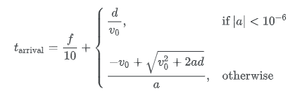
where

2.2 Core Features (Full Model with Anticipation)
To predict expected arrival time, the model incorporates physical and anticipatory features. The list of features that were considered are listed here:
Distance to ball landing spot at time of release.
Orientation angle vs angle to ball: The defender’s facing direction relative to the angle to the ball.
Movement angle vs angle to ball: The defender’s velocity direction relative to the angle to the ball.
Speed at release
Acceleration at release
Player congestion:
Players in Path to Ball: Number of players between the defender and the landing spot.
Players Near Landing Zone: Number of players around the landing spot.
Defender height
Pass length
Distances are computed using Euclidean geometry. Angular variables are normalized to ensure consistent interpretation across the field. Players in Path to Ball is defined as a count of players within a defined path between the player and the ball.
2.3 Reduced Feature Model (No Anticipation)
A reduced model is also trained with the same features, excluding orientation angle vs angle to ball and movement angle vs angle to ball. This model excludes features that can be seen as anticipatory information and focuses only on physical features such as distance, speed, acceleration, and congestion. Comparing the prediction from the full model to this reduced model yields a value explaining how much anticipation effected the defenders' close out effort.
3. Model Results
3.1 Model Selection
Expected arrival time is modeled using a number of supervised machine learning regression models, including Linear Regression, Random Forest, and XGBoost. After comparing the performance (MAE, RMSE, R2) of the three models, XGBoost yields the best results across the board and was selected. XGBoost may outperform linear regression and random forest here because it captures the nonlinear effects of speed, distance, and acceleration, as well as the threshold behaviors in pursuit that simpler models cannot.
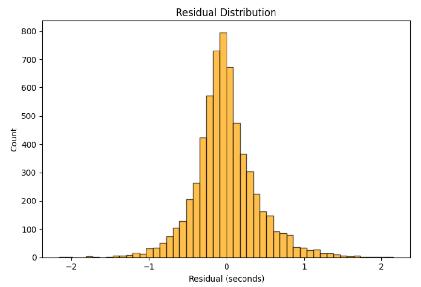
3.2 Model Accuracy
The XGBoost model shows strong alignment between predicted and actual closing times, indicating that the model effectively learns closing behavior from the inputs. It yields an MAE of 0.296 seconds, an RMSE of 0.410 seconds, and an R2 of 0.823. Below is a bar graph showing the residual error distributions, conveying strong model performance.
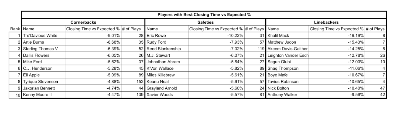
3.3 CTvE Leaderboard
By using our model to predict every defenders expected close out time for every play and comparing that to their actual close out time for each play, their CTvE is calculated. The formula is as follows:
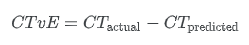
A negative CTvE indicates that a defender overperformed their expected close out time, while a positive CTvE indicates that a defender underperformed their expected close out time.
The CTvE leaderboard below highlights the defenders who, on average, outperform their expected closing time the most. Instead of using raw CTvE, which is useful for evaluating individual plays, the leaderboard uses CTvE% (CTvE divided by predicted close-out time) to normalize for play length and allow for effective comparison of how much time each player is saving.
4. Anticipation
4.1 Anticipation Model vs. No Anticipation Model
The difference in predicted closing time from the full model and the reduced model isolates the effect of anticipation. When orientation and movement angle are included, expected arrival time decreases for defenders who are already aligned with the pass, at release. This effectively credits defenders for pre-trow positioning, route recognition, and early processing.
As expected when removing key features, the anticipation model performed slightly worse than the full model, yielding an MAE of 0.377 seconds, an RMSE of 0.486, and R2 of 0.751,
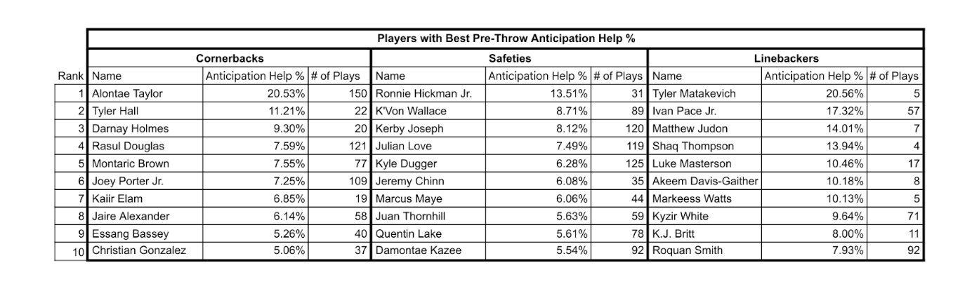
4.2 Anticipation Results
Certain defenders consistently benefit from anticipation adjustments. Their advantage manifests before the ball is even thrown. Below shows the cornerbacks, safeties, and linebackers with the best pre-throw anticipation. Minimum plays were decided by taking the 25th percentile number of plays for each respective position. This threshold will be used for all similar leaderboards.
5. The Three Closing Factors (How/Why Explanations)
This section breaks down a player’s CTvE into three post-throw diagnostic layers.
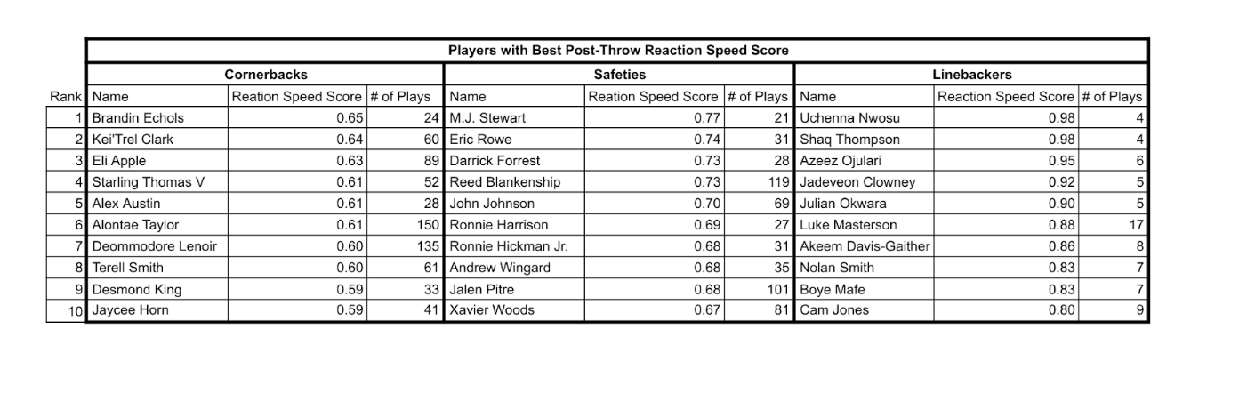
5.1 Reaction Quickness
Reaction quickness is the time from ball release to the defender’s first movement toward the landing spot. For each frame, the angle between the defender’s movement direction and the ball’s landing spot is computed. The threshold for counting a defender as moving towards the ball is a difference in 45 degrees between their movement angle and angle to the ball. This measures recognition skill and processing speed. In order to account for players that never moved towards the ball, but still record raw reaction time (rather than percentage) than can be compared across different play lengths, the reaction speed score was defined as:

where

An easy way to think about this formula is that if a defender’s first movement toward the ball occurs on frame 1, they receive a score of 1.0. For every additional frame before their first movement towards the ball, 0.1 is subtracted from their score. Because the lowest possible score is 0, taking 11 frames (1.1 seconds) or more results in a score of 0.
Below are the players that showed the best reaction speed score.
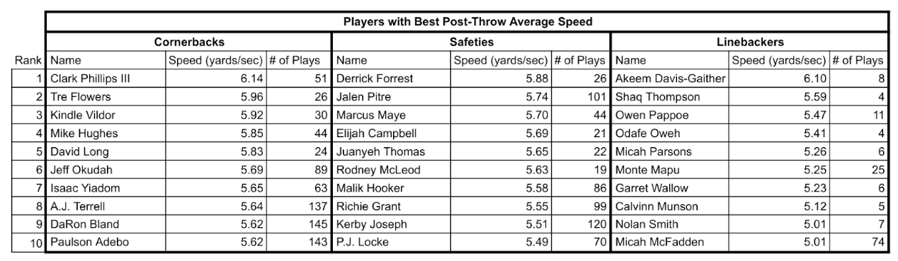
5.2 Speed Profile
Speed is measured in yards per second during the window from ball release to ball arrival. This captures the defender's physical explosiveness. Below are the players that showed the best speed profile.
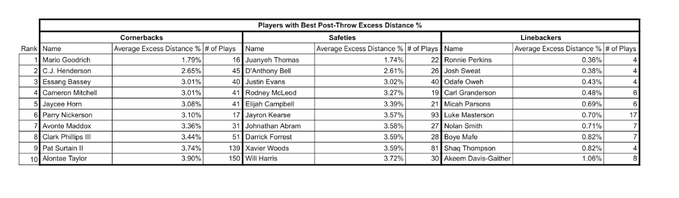
5.3 Path Efficiency
Path efficiency measures the excess distance that a player travels from their start position to their end position. If they travel in a perfectly straight line, their raw excess distance and excess distance percentage would be zero. Below are the players that showed the best path efficiency.
6. Integrating the Models and Factors
6.1 Explaining Over and Underperformance
This section describes and visualizes three plays that illustrate how reaction speed, speed, and path efficiency can each contribute to a positive or negative CTvE.
1. Over Performing (Negative CTvE) due to Elite Reaction Speed
In a game between the Lions and the Bears, Jaylon Johnson is in man coverage against Sam Laporta. Instead of playing Laporta tight, he guards the sideline, knowing that he has safety help over the middle of the field. This cushion that Laporta has tempts Goff to attempt this pass 20 yards downfield.
Johnson instantly reacts to this pass, meaning that even with slow speed and average path efficiency, he is able to achieve a CTvE of -0.47 seconds, leading to an interception.
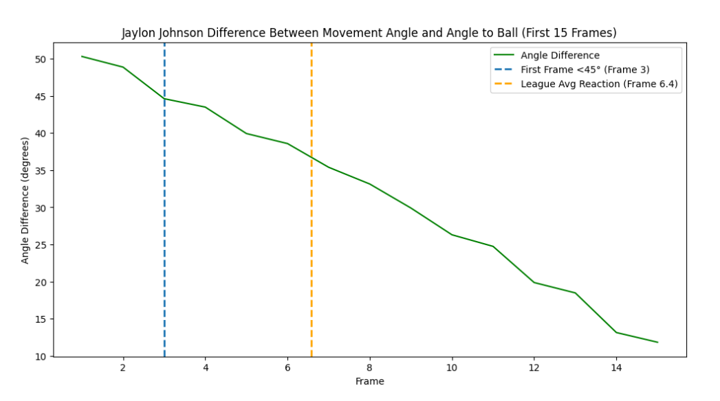
The graph above shows Johnson achieving the angle difference threshold 0.3 seconds after the ball is released. This beats the average defender reaction speed by over 0.3 seconds and was the primary reason for Johnson’s interception.
2. Over Performing (Negative CTvE) due to Elite Speed
In a game between the Patriots and the Bills, Alex Austin is matched up 1-on-1 with Trent Sherfield at the bottom of the screen. Sherfield runs deep toward the middle of the field on a crossing concept with Dalton Kincaid, who cuts to the bottom of the screen. When Allen targets Kincaid, Austin is still covering Sherfield closely, about 10 yards from Kincaid and 17.5 yards from the ball’s landing spot.
Although Austin isn’t the primary defender and isn’t really in a position to make a play on the ball, he averages a speed of around 6.8 yards per second. Even while recording only slightly above average reaction speed score and slightly below average excess distance percentage, his speed allowed him to have a CTvE of -0.1 seconds, leading to an interception.
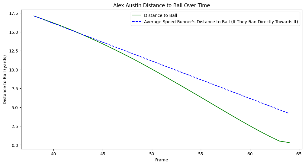
The graph shows Austin’s distance to the ball’s landing zone over time, starting from the moment the ball is released. It also compares his performance to a defender running at average speed directly toward the ball. Even with slightly below-average path efficiency, Austin significantly outperforms the average-speed runner.
3. Under Performing (Positive CTvE) due to Poor Path Efficiency
In a game between the Bengals and the Texans, Mike Hilton is lined up in the slot, shadowing running back Devin Singetary. After Stroud is forced to scramble and throws up a high, wobbly pass for Noah Brown, Hilton finds himself with time to make a play. Although his average reaction speed score and average speed didn’t do him any favors, Hilton’s poor path efficiency led to a CTvE of 0.1 seconds and gave him no chance to contest the catch.
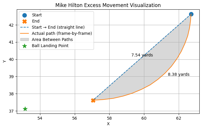
The graph shows the extreme curve in Hilton's approach to the ball’s landing spot, showing that he ran an excess of 0.86 yards to get from his starting point to his ending point. Had he ran those 8.38 yards directly at the ball, Hilton would have been within the catch radius and had a chance to break up the pass.
6.2 Diagnostic Profiles
By looking at the three post-throw factors, players can be grouped into different diagnostic profiles that highlight their strengths and weaknesses. Below are some example profiles, and high-profile players that fit the profiles:
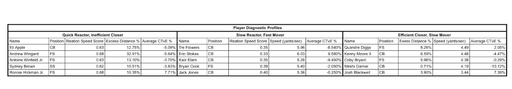
Each player produces a unique combination of reaction, speed, and path efficiency scores, which together determine their ability to reach the ball on time. By analyzing these metrics, teams gain a more complete understanding of a player’s CTvE. Some players of all profiles achieve high CTvE percentages, while others perform poorly. This demonstrates that defenders with specific strengths and weaknesses can still be effective when properly utilized, but may become liabilities if deployed incorrectly. Further research could examine when defenders of each profile tend to have negative or positive CTvE, such as in man versus zone coverage, defending the X/Y/Z receiver, on the sidelines versus over the middle, or on deep routes versus short passes. This insight allows coaches to identify which players are most suitable for different roles.